From Hypothesis to Conclusions: A Deep Dive into T-Tests for Data-Driven Analysis

In our journey as analysts, our goal is to harness the power of data to bring intelligence to the decision-making table. We're not just number-crunchers; we're storytellers who strive to use data that can guide our stakeholders to make informed decisions based on evidence rather than intuition.

Hypothesis testing, including t-tests, is one such method that can equip us all as analysts to measure impact, provide evidence and enable future decision-making. T-test is one of the most commonly used Hypothesis tests in statistics and hence the choice for this blog. With the t-test, we can answer crucial questions like, "Does this intervention truly make a difference?" or "Is this new strategy really paying off?"

So let's understand what is a T-test, what are its assumptions, what are its types and which type is suited to use when. We will solely focus on understanding the concept in this blog rather than code because with tools like Chat GPT, coding is a cinch.

In the previous blog, I already covered what is hypothesis testing, so let's dive straight into what is a t-test in this blog.

What is a T-Test?

A T-test is a measure that allows us to identify whether there is a statistically significant difference between the means of two groups. It rules out whether the mean difference could have happened by chance.

For example, let's say a company wants to determine if there is a significant difference in the average sales performance between two different sales teams or if it happened just by chance. They can perform a T-test to validate this hypothesis.

Assumptions of T-test?

1). The data should be continuous

The T-test is not suited for categorical data.

2). The data should be randomly sampled from a population

Random sampling ensures there is no bias and the sample is representative of the population. By ensuring that the sample is representative of the population, the findings from the sample can be generalized back to the population with greater confidence.

3). There is homogeneity of variance

Similar variability in each group ensures that differences observed between groups are not due to differences in data spread, enabling fair comparisons and accurate conclusions about group differences. Essentially, you need to ensure that you are comparing apples with apples.

4). The distribution is approximately normal.

A normal distribution indicates that most data points cluster around the mean, with fewer data points towards the extremes. When data is approximately normally distributed, it allows for more reliable statistical analyses and interpretations, ensuring that the results are valid and trustworthy.

What are the different types of T-tests?

There are three different types of T-tests:

1. One-Sample T-test/Student's T-test
2. Two-Sample T-test/Independent Sample T-test
3. Paired T-test/Dependent Sample T-test

Let's try to make sense of the three types with the example below:

USE CASE:

Let's collect data to validate Alicia's claim and also understand the types of T-tests at the same time.

CASE 1:

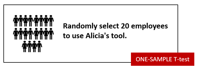
In a one-sample t-test, we compare the mean of a single group/sample with a KNOWN mean.

• Null Hypothesis (H0): The mean reduction in admin work hours using Alicia's tool is not significantly different from 10 hours.
• Alternative Hypothesis (H1): The mean reduction in admin work hours using Alicia's tool is significantly different from 10 hours.

CASE 2:

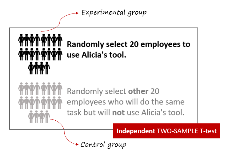
Independent Sample T-test compares the difference in the mean between two groups/samples. We need to ensure the groups are independent of each other, hence we choose completely different 20 other employees for the control group.

• Null Hypothesis (H0): There is no significant difference in the mean reduction in admin work hours between the group using Alicia's tool and the control group (not using the tool).
• Alternative Hypothesis (H1): There is a significant difference in the mean reduction in admin work hours between the group using Alicia's tool and the control group.

Case 3:

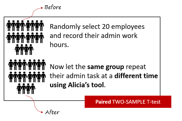
Paired sample t-test compares the mean of the same group at different times. It is essentially a before and after comparison of one group.

• Null Hypothesis (H0): There is no significant difference in the mean reduction in admin work hours between the paired groups (before and after using Alicia's tool).
• Alternative Hypothesis (H1): There is a significant difference in the mean reduction in admin work hours between the paired groups.

Interpretation of Results:

A t-test return two values, a T-score and a p-value.

A T-score indicates the ratio between the difference between two groups and the difference within the groups.

• Larger T-score = more difference between groups.
• Smaller T-score = more similarity between groups.

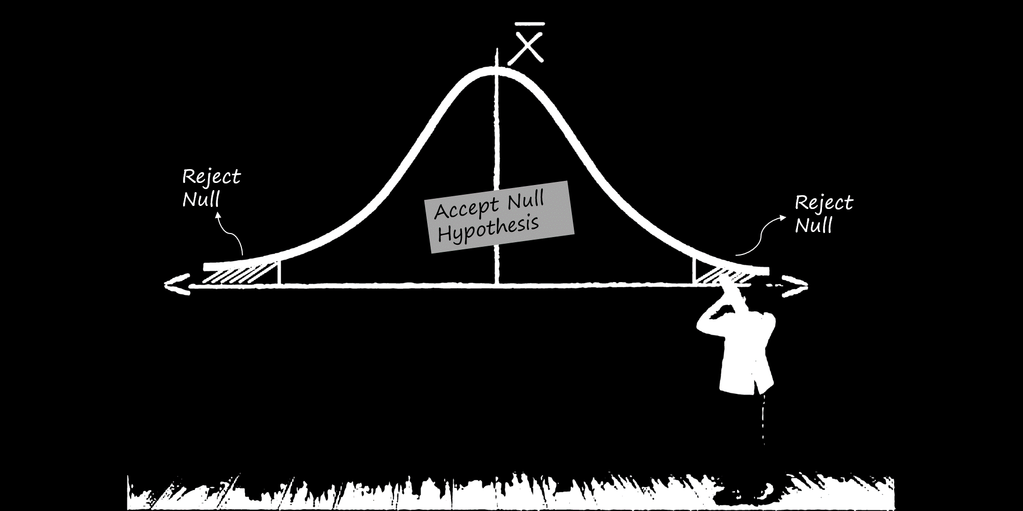
A p-value tells us the probability of the outcome happening by chance. In all three cases, if the p-value is less than the chosen significance level (e.g., 0.05), we reject the null hypothesis and conclude that Alicia's claim is right - there is a significant difference in the mean reduction in admin work hours.

Example - So, let's say after performing a t-test, we get a p-value of 0.02 (2%), it means if we were to repeat the experiment several times and assume that Alicia's claim was true (null hypothesis is true), then the probability of it being true is just 2%. That is why we reject the null hypothesis when the p-value is less than 0.05 (chosen significance level).

To summarise,

One Tail Test vs Two Tail Test

Before defining the hypothesis or collecting data, there is another question that we need to ask ourselves. Do we want to perform one-tail t-test or two-tail t-test?

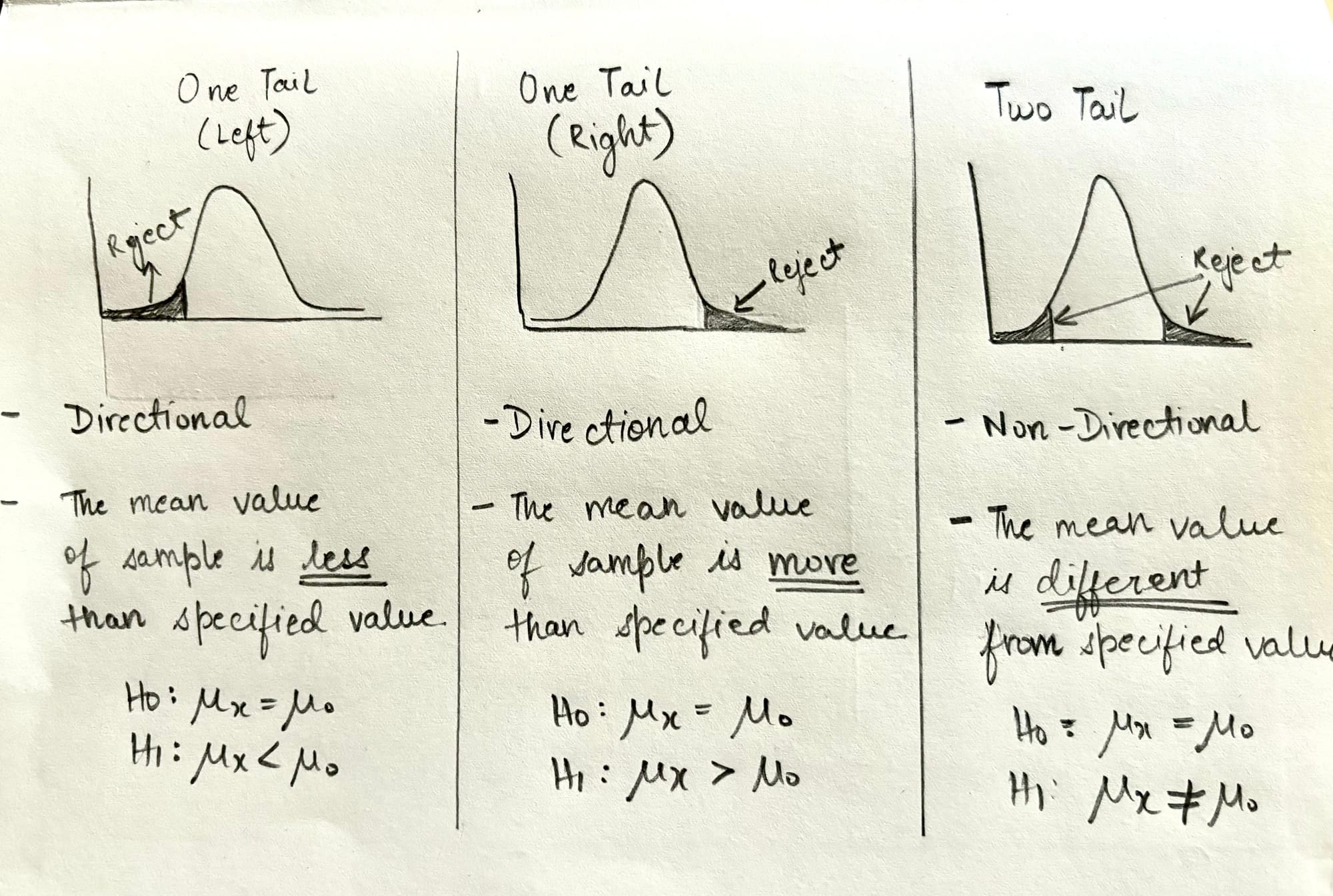
In a one-tail t-test, we're interested in whether a sample mean is significantly greater or significantly less than a hypothesized population mean, but not both.

In a two-tail t-test, we're simply interested in whether a sample mean is significantly different than a hypothesized population mean. It can be less, it can be more, we are not sure.

Can you tell which type did we choose in Alicia's case? - We performed a two-tail t-test because we were interested to see if the sample mean was significantly different; it could be less, it could be more.

It would have been one-tail if our alternate hypothesis was - the mean reduction in admin work hours using Alicia's tool is significantly less than 10 hours.

Let's summarise: