The Statistical Frontier of the Global AI Race Through Hypothesis Testing
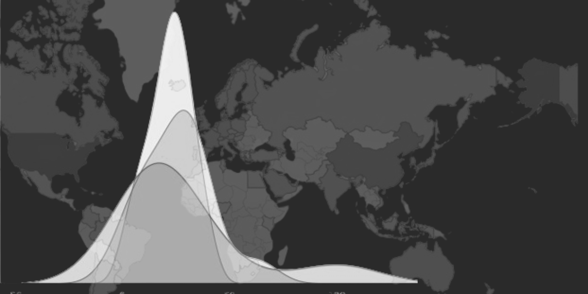
In today's hyper-connected world, the race for AI dominance is heating up like never before. In this relentless pursuit of AI supremacy, all the nations are making waves with groundbreaking research, bold initiatives, and ambitious investments, challenging the traditional notion of AI dominance.
So I ask you today, which among the three regions, is leading the AI race according to you?
- AMER: North, Central, and South America.
- APAC: Asia and Pacific.
- EMEA: Europe, the Middle East, and Africa.
If you are thinking AMER, well then,

Before jumping to any conclusion, let's try to find some significance in our claim.
Tortoise Media launched something known as the AI Index which helps to make sense of AI globally. Essentially, their Global AI Index benchmarks 62 countries in three main areas:
- Investment - how much money countries are putting into AI;
- Innovation - how innovative they are with it, and
- Implementation - how well they're using it in real life.
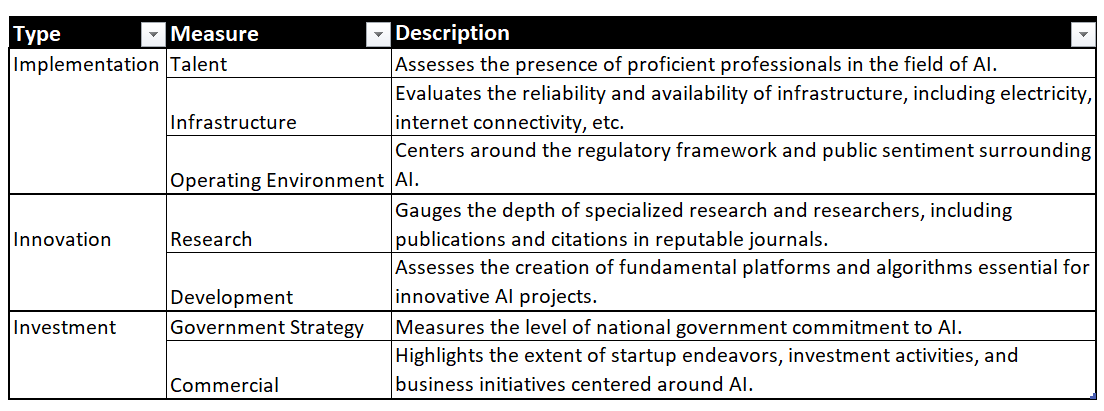
They launched the AI index in 2019 and this is the fourth time they've done this ranking. They base their ranking on 7 main indicators: Talent, Infrastructure, Operating Environment, Research, Development, Government Strategy, and Commercial aspects of AI. If you are curious to know more about their methodology for calculating sores, find out here.
In this blog, with the help of AI index data obtained from Kaggle, we'll channel our inner statistician to investigate: If there is a statistically significant difference between the AI scores of the three regions.
But how do we do that - Enters Hypothesis Testing.
Before jumping into the world of Inferential Statistics, let's have a quick look at our data and understand it better with some basic data exploration.
Exploratory Data Analysis
I have used Python in Databricks Notebook for this analysis, however, you can stick to any language and platform you are comfortable with.
AI Index Data consists of 62 rows and 13 columns. Here is how the top 5 rows look like:

Each row in the dataset represents a different country, along with its scores ranging from 1 to 100 across seven important areas. Additionally, there are columns indicating the total score and several categorical variables that categorize the countries into five regions, five clusters, three income groups, and four types of political regimes.
To understand the metrics better, below is a data dictionary for quick reference.
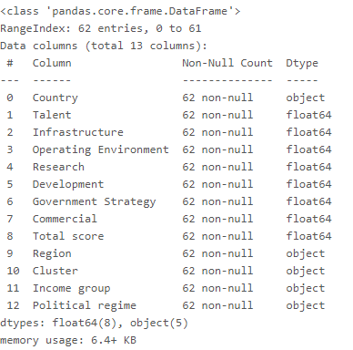
The dataset contains no missing values and data types look correct.
For the numeric variables, let's look at their basic descriptive statistics:

The minimum and the maximum values are between 0 to 100 for all the variables so the scale of values is correct.
Commercial, Development, and Talent have low average scores. Perhaps this is due to the nascent stage of AI adoption and innovation, possibly due to limited investment, research, and skilled workforce availability in most nations. Conversely, Operating Environment, Infrastructure, and Government Strategy have high average scores. This can be indicative of robust support structures, including favourable regulatory environments, advanced technological infrastructure, and government policies incentivizing AI development.
Let's check if there is a correlation between the variables.
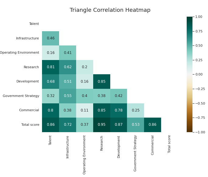
Clearly, there exists a positive correlation among all variables, as growth in one area tends to correspond with growth in others. Talent exhibits a strong correlation with research, which is unsurprising given that increased talent often leads to better and more advanced research. Moreover, research shows a high correlation with both commercial and development scores, indicating a direct relationship wherein more research fosters greater development, subsequently driving investment and business initiatives in artificial intelligence.
Now, let's also take a quick look at our categorical variables.
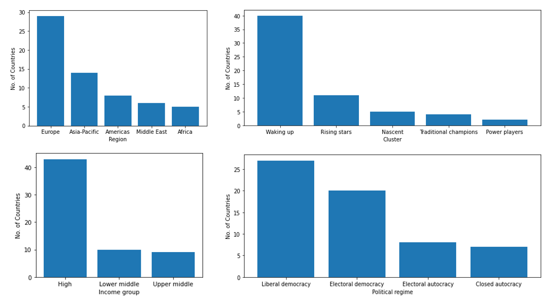
In this analysis, the countries USA and China are classified as power players, while the UK, Canada, Germany, and France are categorized as traditional players. Moreover, out of the 62 countries in the dataset, 43 fall under the high-income level category.
It would be interesting to look at the distribution of different scores within each category. However, for this analysis, we will stick to two variables, total score and region and we will group the five regions into three: the Americas (AMER), Asia-Pacific (APAC), and Europe, Middle East, and Africa (EMEA).
Now through density plots and box plots, let's uncover insights into the variations in total scores across these three regions.
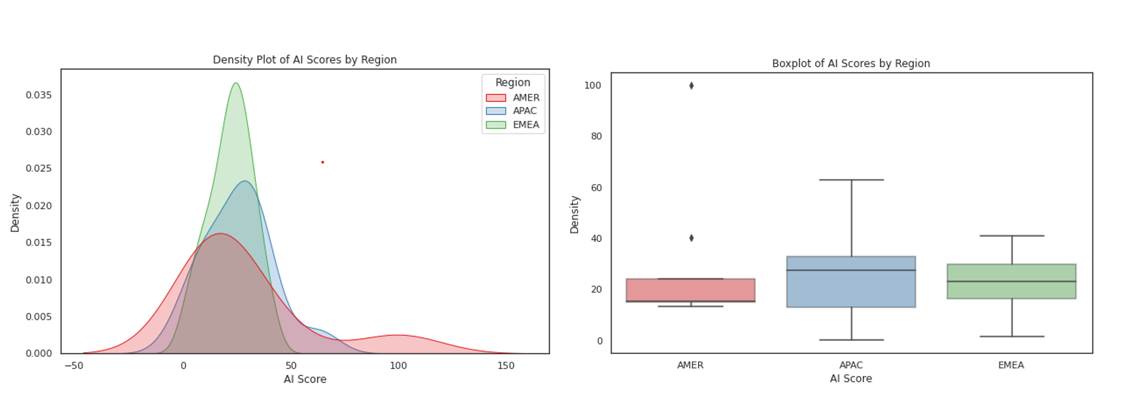
Upon initial inspection, the distribution of AI scores across the three regions appears to have relatively low dispersion, with the majority falling within the range of 10 to 30. Notably, the Americas exhibit a few distinct outliers and seem to have a highly right-skewed distribution, as evidenced by the heavy tail. APAC also demonstrates a slight right skewness but lacks any clear outliers. In contrast, the AI scores in EMEA appear to follow a fairly normal distribution.
With this preliminary understanding of our data, let's delve into our analysis and perform hypothesis testing to determine whether there exists a statistically significant difference in AI scores among the three regions.
But first, let me try and explain what is hypothesis testing in the simplest and shortest possible way.
What is Hypothesis Testing?
Imagine you're a detective trying to solve a mystery. You have a suspect, but you need evidence to prove their guilt or innocence. Hypothesis testing is like being that detective in the world of statistics.
You start with two ideas: the null hypothesis (H0) which says there's no difference (not guilty - the default assumption), and the alternative hypothesis (H1) which says there is a difference (guilty).
To test these hypothesis, you collect clues (data) from a sample. You then unleash your statistical toolbox to crunch those numbers and calculate a "test statistic" – basically, a score that tells you how likely it is that your sample data supports the null hypothesis.
Next comes the moment of truth: comparing your test statistic to a magical number called the p-value. This number tells you the probability of seeing your results just by random chance. If this probability is very low (typically less than 0.05), you have a smoking gun! You reject the null hypothesis and accept the alternative – your suspect (or variable) is guilty (or different)!
But if the p-value is higher than your chosen significance level, it's like saying, "Hmm, not enough evidence." You can't make a strong case, so you stick with the null hypothesis – your suspect walks free (or your variables are deemed similar).
In the end, hypothesis testing is your statistical Sherlock Holmes, helping you decide if the evidence in your data is strong enough to support your theories. It's a method that turns numbers into conclusions and stats into stories.
So in our case,
Null Hypothesis: There is no significant difference in the AI scores of the three regions.
Alternation Hypothesis: There is a significant difference in the AI scores of the three regions.
Now that we have established our null and alternate hypothesis, the next step is to decide which test statistic to use. There are several statistical tests which are available such as T-Test, Z-Test, ANOVA, and many more. So how do we decide which one to use?
Choosing the right statistical test
Let's understand them very briefly.
T-Test: It is used to compare the mean between two groups (samples) that have a small sample size (typically, n<30).
Z-Test: It is used to compare the mean between two groups (samples) but the samples have a large size.
ANOVA (Analysis of Variance): It is an extension of the T-Test but is used to compare the mean between three or more groups.
The explanation above is merely touching the surface of these tests. Each one is a vast topic in itself in statistics and goes into much more detail. I will cover more about them in a separate blog. For now, this explanation is enough for us to understand that our choice of test statistic would be ANOVA because we have 3 regions (3 samples) that we want to compare.
Let's go ahead and run ANOVA.
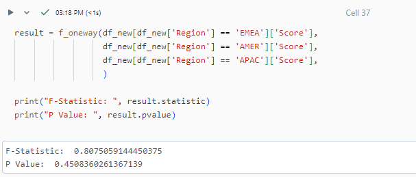
The p-value is 0.45 which is greater than the 0.05 (assumed critical value in this case). This means we cannot reject the null hypothesis implying there is no significant difference in the AI sores of the three regions.

Can we trust this result? NO.
Why? Because every test statistic has its own assumptions that need to be tested on the data. If the data does not meet the assumptions, that means we cannot perform that test statistic or we need to transform our data so that it meets the assumption of the analysis.
Validating Assumptions
For ANOVA, there are two main assumptions:
1). Normality
The data should be normally distributed and we can check for Normality in two ways:
Method 1: Plotting a density curve and analysing the shape of the AI scores.
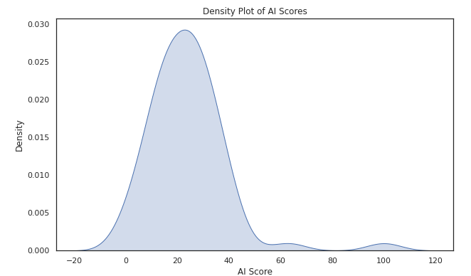
Conclusion: Visually, the data does not look normally distributed. It is right-skewed meaning that it has a long tail on the right and most of the data is concentrated towards the left. It has a peak at around 23.
Method 2: Shapiro-Wilk Test of Normality (for smaller samples <50) or Kolmogorov-Smirnov Test of Normality (for sample size >50)
We will perform the Kolmogorov-Smirnov Test of Normality since our sample size is 62. It assumes that the data is normally distributed.

Conclusion: A p-value less than 0.05 means we can reject our null hypothesis. So according to this test also, the data is not distributed normally.
2). Homogeneity of Variance
Homogeneity of Variance means that the variance among the groups should be approximately equal. To check for this assumption, we can make a box plot or a violin plot, as we did in our exploratory analysis. But a more accurate way to test for homogeneity of variance is by performing Levene's Test. It's the default assumption the variance between groups is not equally distributed.

Conclusion: The p-value is greater than 0.05, hence we cannot reject the null hypothesis. Hence, we can say that our data violates the assumption of homogeneity of variance.
NOW WHAT? Our data is neither normal nor homogenous.

This means we were wrong in our choice of performing ANOVA. That means before choosing a test statistic, YOU MUST CHECK THE ASSUMPTIONS.
Well, fear not. Statistics has a solution to this.
We will need to use a non-parametric alternative called Krukal Wallis H-Test.
Kruskal Wallis H-Test
Kruskal Wallis is simply a non-parametric equivalent of one-way ANOVA. It assesses whether the medians of two or more groups are equal or not.
Contrary to ANOVA, it has more flexible assumptions. It assumes the data is not normal and is not homogeneous. Both of which are true in our case. So let's go ahead and perform this test on AI scores.

Since our p-value is more than the chosen significance level of 0.05, we cannot reject the null hypothesis. Hence we conclude that there are no significant differences among the AI Scores for three regions.
Conclusion:
In the ever-evolving landscape of artificial intelligence, our quest for understanding the dynamics of global AI dominance led us through a journey of data exploration and statistical analysis. While our initial curiosity hinted at potential disparities among regions, rigorous hypothesis testing revealed a different narrative. Despite the nuanced differences in AI scores across the Americas, Asia-Pacific, and Europe, Middle East, and Africa, our statistical inquiries ultimately affirmed a lack of significant distinctions among them. As we conclude this chapter, let us remain vigilant in our pursuit of knowledge, ever ready to challenge assumptions and embrace the complexities of the AI landscape. After all, in the realm of technology and innovation, every insight gained brings us closer to unlocking the boundless potential of artificial intelligence.

